Introduction
In this blog post, I share a complete overview of a deep learning-based medical imaging project focused on detecting leprosy from skin images. We use a blend of advanced CNN architectures like EfficientNet, VGG16, MobileNet, and Xception, all optimized through hinge loss—a method inspired by SVMs—to accurately distinguish between leprosy and non-leprosy images.
🔗 Project Links
- GitHub Repository: Leprosy Detection Project
- Dataset: Leprosy Dataset
Dataset Overview
The dataset is structured into two classes:
-
Leprosy (Label 1)
Images show visible symptoms of leprosy.
Folder:new_train/Leprosy -
Non-Leprosy (Label 0)
Images depict healthy skin.
Folder:new_train/Non_Leprosy
Data Preprocessing
We applied several preprocessing steps to ensure consistent input and enhance generalization:
- Resizing all images to
(256, 256)pixels. - RGB Conversion using
Image.open(...).convert("RGB"). - Random Saturation variation using HSV channel manipulation.
- Clean Directory Handling with
os.path.join()and directory checks. - Systematic File Renaming to avoid duplicates and maintain order.
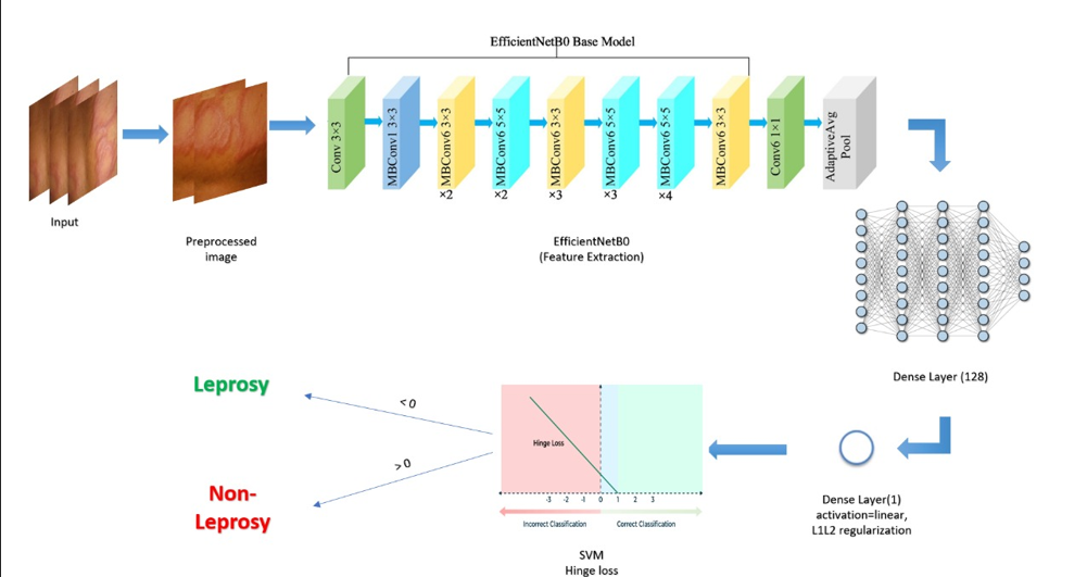
Modeling Approach
We tested several CNN architectures using transfer learning:
-
EfficientNetB0
Pre-trained model fine-tuned for our binary classification task. -
VGG16
Simple and widely used; enhanced with hinge loss and linear output. -
MobileNet
Lightweight and ideal for embedded/mobile applications. -
Xception
Leverages depthwise separable convolutions for efficiency.
All models pass through a final Dense layer (linear activation) with L2 regularization and use hinge loss to enforce margin-based classification—akin to SVMs.
If final output > 0 → Leprosy
If final output < 0 → Non-Leprosy
Why These Models?
- Transfer learning leverages pre-trained features on ImageNet.
- EfficientNet adapts quickly with minimal training data.
- Hinge loss maximizes separation margin between classes.
- L2 regularization prevents overfitting.
Training Strategy
- Train/Test Split: 80% training, 20% testing
- Optimizer: Adam with learning rate 0.01
- Loss: Hinge loss
- Regularization: L2
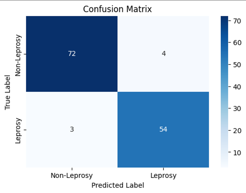
Evaluation Metrics
| Metric | Value |
|---|---|
| Precision | 0.931 |
| Recall | 0.947 |
| F1 Score | 0.939 |
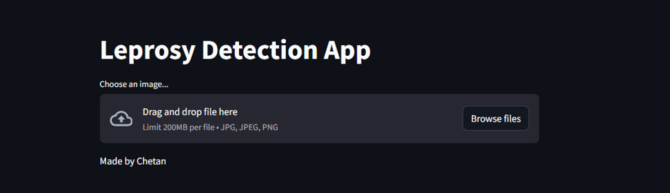
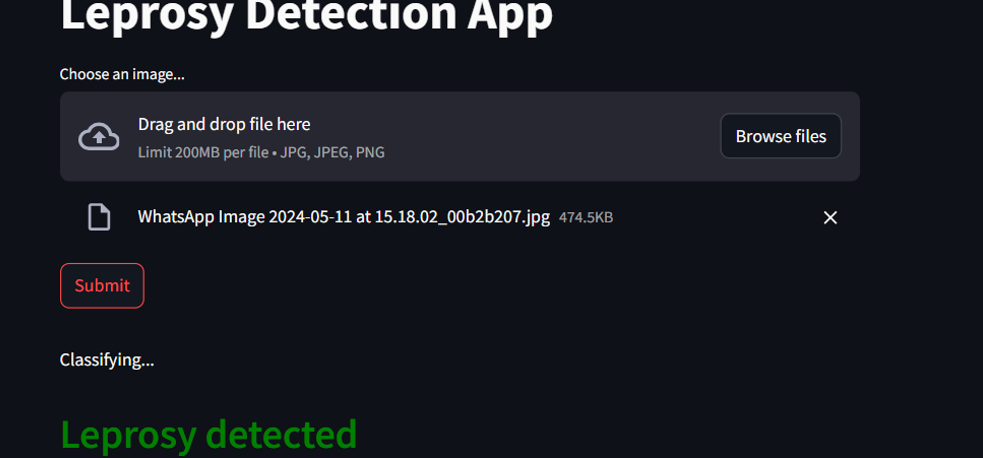
Hosting the Model in Google Colab
-
Upload the files:
modelapp.pysvm_in_cnn.h5run.sh
-
Run the command in your Colab notebook.
-
Click the provided URL.
-
Use your IP address as the password.
Final Thoughts
This project combines the strengths of traditional SVM theory and modern deep learning architectures. It’s an ideal example of how even small datasets can yield accurate results with the right preprocessing, model selection, and evaluation pipeline.
👨⚕️ Bridging the gap between machine learning and healthcare—one pixel at a time.