A Neural Network from Scratch

import matplotlib.pyplot as plt
from sklearn.datasets import make_circles
from sklearn.model_selection import train_test_split

# Create a dataset with 10,000 samples.
X, y = make_circles(n_samples = 10000,
                    noise= 0.05,
                    random_state=26)

X_train, X_test, y_train, y_test = train_test_split(X, y, test_size=.33, random_state=26)

# Visualize the data.
fig, (train_ax, test_ax) = plt.subplots(ncols=2, sharex=True, sharey=True, figsize=(10, 5))
train_ax.scatter(X_train[:, 0], X_train[:, 1], c=y_train, cmap=plt.cm.Spectral)
train_ax.set_title("Training Data")
train_ax.set_xlabel("Feature #0")
train_ax.set_ylabel("Feature #1")

test_ax.scatter(X_test[:, 0], X_test[:, 1], c=y_test)
test_ax.set_xlabel("Feature #0")
test_ax.set_title("Testing data")
plt.show()

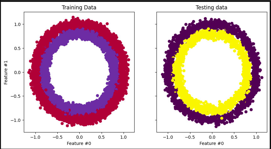
• This code imports the necessary libraries for creating a dataset, splitting it into training and testing sets, and visualizing the data.

• The make_circles function from sklearn. datasets are used to create a dataset with 10,000 samples.

• The n_samples parameter specifies the number of samples to generate, noise adds random noise to the data, and random_state sets the seed for the random number generator to ensure reproducibility.

• The train_test_split function from sklearn.model_selection is used to split the dataset into training and testing sets.

• The test_size parameter specifies the proportion of the dataset to include in the testing set, and random_state sets the seed for the random number generator to ensure reproducibility.

• The fig, (train_ax, test_ax) = plt.subplots(ncols=2, sharex=True, sharey=True, figsize=(10, 5)) line creates a figure with two subplots, one for the training data and one for the testing data.

• The ncols=2 parameter specifies the number of columns in the figure, sharex=True and sharey=True ensure that the x and y axes are shared between the subplots, and figsize=(10, 5) sets the size of the figure.

• The train_ax.scatter and test_ax.scatter functions are used to plot the training and testing data, respectively.

• The c parameter specifies the color of the points based on the target variable (y_train or y_test).

• The set_title, set_xlabel, and set_ylabel functions are used to set the title and axis labels for the training data subplot.

• Finally, plt.show() is used to display the figure.

import warnings
warnings.filterwarnings("ignore")

!pip install torch -q

import torch
import numpy as np
from torch.utils.data import Dataset, DataLoader

# Convert data to torch tensors
class Data(Dataset):
   def __init__(self, X, y):
       self.X = torch.from_numpy(X.astype(np.float32))
       self.y = torch.from_numpy(y.astype(np.float32))
       self.len = self.X.shape[0]
      
   def __getitem__(self, index):
       return self.X[index], self.y[index]
  
   def __len__(self):
       return self.len
  
batch_size = 64

# Instantiate training and test data
train_data = Data(X_train, y_train)
train_dataloader = DataLoader(dataset=train_data, batch_size=batch_size, shuffle=True)

test_data = Data(X_test, y_test)
test_dataloader = DataLoader(dataset=test_data, batch_size=batch_size, shuffle=True)

# Check it's working
for batch, (X, y) in enumerate(train_dataloader):
   print(f"Batch: {batch+1}")
   print(f"X shape: {X.shape}")
   print(f"y shape: {y.shape}")
   break

• It defines a class called Data that converts input data into torch tensors.
• The class has three methods: init that initializes the class with input data, getitem that returns the data at a specific index, and len that returns the length of the data.
• The code then instantiates training and test data using the Data class and DataLoader.
• The DataLoader is used to load the data in batches of size 64 and shuffle the data.
• Finally, the code checks if the DataLoader is working by printing the shape of the first batch of data.
• The warnings library is used to ignore any warnings that may arise during the execution of the code.
• The !pip install torch -q command installs the torch library without displaying any output.
• The numpy library is used to convert input data into numpy arrays before converting them into torch tensors.
• Overall, this code converts input data into torch tensors and loads them into batches using DataLoader for efficient training and testing of machine learning models.

import torch
from torch import nn
from torch import optim

input_dim = 2
hidden_dim = 10
output_dim = 1

class NeuralNetwork(nn.Module):
   def __init__(self, input_dim, hidden_dim, output_dim):
       super(NeuralNetwork, self).__init__()
       self.layer_1 = nn.Linear(input_dim, hidden_dim)
       nn.init.kaiming_uniform_(self.layer_1.weight, nonlinearity="relu")
       self.layer_2 = nn.Linear(hidden_dim, output_dim)
      
   def forward(self, x):
       x = torch.nn.functional.relu(self.layer_1(x))
       x = torch.nn.functional.sigmoid(self.layer_2(x))

       return x
      
model = NeuralNetwork(input_dim, hidden_dim, output_dim)
print(model)

• This code defines a neural network model using the PyTorch library.
• First, the necessary libraries are imported: torch, nn (short for neural network), and optim (short for optimizer).
• Next, the input, hidden, and output dimensions of the neural network are defined.
• Then, a class called NeuralNetwork is defined, which inherits from the nn.Module class.
• This class has an init method that initializes the layers of the neural network.
• The first layer is a linear layer (nn.Linear) that takes in the input dimension and outputs to the hidden dimension.
• The weights of this layer are initialized using the Kaiming uniform initialization method with a ReLU nonlinearity.
• The second layer is another linear layer that takes in the hidden dimension and outputs to the output dimension.
• The forward method of the NeuralNetwork class defines the forward pass of the neural network.
• It takes in an input tensor x and passes it through the first layer with a ReLU activation function (torch.nn.functional.relu).
• The output of this layer is then passed through the second layer with a sigmoid activation function (torch.nn.functional.sigmoid).
• The final output of the neural network is returned.
• Finally, an instance of the NeuralNetwork class is created with the specified input, hidden, and output dimensions, and the model is printed to show the structure of the neural network.

learning_rate = 0.1

loss_fn = nn.BCELoss()

optimizer = torch.optim.SGD(model.parameters(), lr=learning_rate)

• The code also defines the loss function as Binary Cross Entropy (BCE) Loss, which is commonly used for binary classification problems.
• Finally, the code initializes the optimizer as Stochastic Gradient Descent (SGD) with the model parameters and the learning rate as inputs.
• The optimizer is responsible for updating the model parameters during training to minimize the loss function.

num_epochs = 100
loss_values = []


for epoch in range(num_epochs):
   for X, y in train_dataloader:
       # zero the parameter gradients
       optimizer.zero_grad()
      
       # forward + backward + optimize
       pred = model(X)
       loss = loss_fn(pred, y.unsqueeze(-1))
       loss_values.append(loss.item())
       loss.backward()
       optimizer.step()

print("Training Complete")

• This code trains a machine learning model using a training dataset.
• The first line sets the number of epochs to 100.
• An epoch is a complete pass through the entire training dataset.
• The for loop iterates through each epoch.
• Within each epoch, the for loop iterates through each batch of data in the train_dataloader.
• The optimizer.zero_grad() line sets the gradients of all model parameters to zero.
• This is necessary because PyTorch accumulates gradients by default, so we need to reset them before each iteration.
• The pred = model(X) line computes the model’s predictions for the input data X.
• The loss = loss_fn(pred, y.unsqueeze(-1)) line computes the loss between the model’s predictions and the true labels y.
• The unsqueeze(-1) method adds an extra dimension to y to match the shape of pred.
• The loss_values.append(loss.item()) line adds the current loss value to a list of loss values.
• The loss.backward() line computes the gradients of the loss with respect to all model parameters.
• The optimizer.step() line updates the model parameters based on the computed gradients.
• After all epochs and batches have been processed, the code prints “Training Complete”.

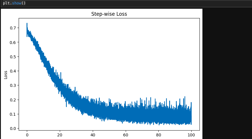
step = np.linspace(0, 100, 10500)

fig, ax = plt.subplots(figsize=(8,5))
plt.plot(step, np.array(loss_values))
plt.title("Step-wise Loss")
plt.xlabel("Epochs")
plt.ylabel("Loss")
plt.show()

!{image

• This code creates a plot of the loss values over a range of steps or epochs.
• First, it creates an array of 10500 evenly spaced values between 0 and 100 using the np.linspace() function and assigns it to the variable step.
• Then, it creates a figure and axes object using plt.subplots() and sets the size of the figure to 8 inches by 5 inches.
• Next, it plots the loss_values array against the step array using plt.plot().
• It sets the title of the plot to “Step-wise Loss” using plt.title(), the x-axis label to “Epochs” using plt.xlabel(), and the y-axis label to “Loss” using plt.ylabel().
• Finally, it displays the plot using plt.show().
• Note that this code assumes that loss_values is a list or array of the same length as step containing the loss values at each step/epoch.

import itertools    
with torch.no_grad():
   y_pred = []
   y_test = []
   total = 0
   correct = 0
   for X, y in test_dataloader:
       outputs = model(X)
       predicted = np.where(outputs < 0.5, 0, 1)
       predicted = list(itertools.chain(*predicted))
       y_pred.append(predicted)
       y_test.append(y)
       total += y.size(0)
       correct += (predicted == y.numpy()).sum().item()

print(f'Accuracy of the network on the test instances: {100 * correct // total}%')