Introduction
Let’s dive into the world of simple linear regression, a fundamental statistical technique used to model the relationship between two quantitative variables.
The Problem
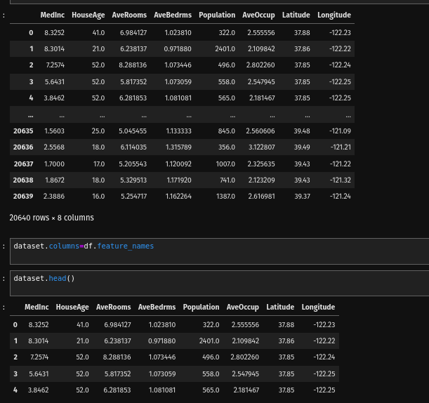
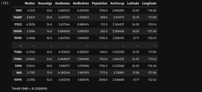
Our goal is to predict housing prices in California based on various factors such as location, median income, housing density, and more. By understanding the relationship between these variables and housing prices, we can provide valuable insights to stakeholders in the real estate industry.
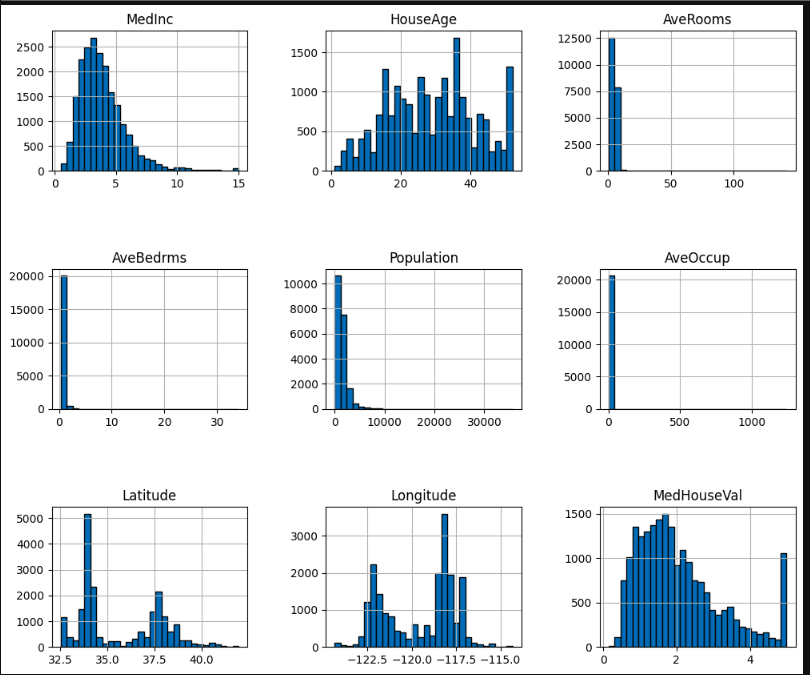
Explore the Data
Perform exploratory data analysis (EDA) to gain insights into the dataset. Visualize key variables using scatter plots, histograms, and correlation matrices to understand their distributions and relationships.
Train the model
regression = LinearRegression()
regression.fit(X_train,y_train)
Here we are fitting the model using Linear Regression
Evaluate the model
We evaluate the performance of the model using metrics such as Mean Squared Error (MSE) and Ridge Regressor
mse = cross_val_score(regression,X_train,y_train,scoring="neg_mean_squared_error", cv = 10)
ridgecv = GridSearchCV(ridge_regressor,parameters,scoring = 'neg_mean_squared_error', cv = 5)
Make Prediction
Now we predict the result using
reg_pred = regression.predict(X_test)
ridge_pred = ridgecv.predict(X_test)
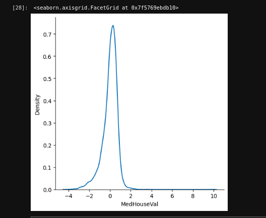
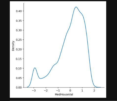
Visualize the data
We visualize the data using seaborn, displt function